2 formulas to calculate age from DOB Google Sheets

Mastering Google Sheets is essential for maximizing productivity while minimizing frustration. But don’t worry if you’re struggling with converting a date of birth (DOB) to age. By the time you’re done reading this guide, you’ll calculate any age in years, months, or even days.

This is a fantastic feature for maintaining databases or data entry involving extensive lists of DOB. The formulas you’re about to learn greatly enhance data analysis and reporting capabilities.

However, like many Sheets functions, converting a birth date isn’t that obvious. We’ll guide you through the process of converting DOB to age in your Google sheet.

Tired of wasting hours navigating Google Sheets' complex functions? Automate your workflows with Bardeen. Download now, save time today!

How to convert a birth date to age in Google Sheets

Converting a birth date to age in Google Sheets is achieved using one of these methods:

• the DATEDIF and TODAY() combination of functions
• the YEARFRAC function

For detailed age statements, both formulas can also be expanded to include years, months, and days, with the option to calculate age across multiple rows using ARRAYFORMULA.

Instead of manually calculating age from a birth date, you can use Bardeen to automate enriching and updating data in Google Sheets. Bardeen can automatically calculate age from DOB and update rows with the age:

Enrich and update leads from a Google Sheet, when new row is added [Beta]

Try it

Both functions can compute the current age based on the DOB provided, but they differ in complexity and the type of result they return:

• DATEDIF calculates the total number of days, months, or years between two dates
• the YEARFRAC function calculates the fraction of a year between two given dates

Bardeen can also classify, qualify or enrich rows in other ways to add more context to your Google Sheet:

Classify past emails and save to Google Sheets

Try it

Qualify leads from meeting notes in a Google Sheet

Try it

Enrich contacts using names and company information in Google Sheets

Try it

Using DATEDIF to calculate age in Google Sheets

The most commonly used formula for calculating age in Google Sheets is the DATEDIF function. It requires just three parameters:

• the start date (DOB)
• the end date (usually the current date)
• the unit of measurement (years, months, or days)

The basic syntax for calculating age in years is: '=DATEDIF(start_date, end_date, "Y")'

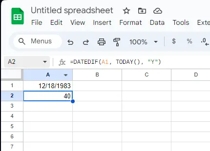
To use the current date as the end date, you can utilize the TODAY() function, making the formula: '=DATEDIF(A1, TODAY(), "Y")'

Assume the DOB is in cell A1; this formula will return the age (in full years) in the blank cell below it.

Bardeen can help automate importing data from various sources into Google Sheets, saving you time and effort. Try these playbooks:

Get data from the currently opened Youtube history page and save to Google Sheets

Try it

Copy all emails from a timeframe to Google Sheets, saving all attachments in Google Drive

Try it

Do you often use such functions manually? Then, you probably understand the level of attention needed when entering commands. Even a single error can disrupt the entire function, so why not leverage workflow automation? It can do wonders for your personal productivity.

Bardeen can also help you use data in Google Sheets to generate personalized content, further automating your workflows:

Create personalized recruiting emails using LinkedIn profile links in Google Sheets

Try it

Using YEARFRAC to calculate age in Google Sheets

The YEARFRAC function's ability to calculate the fraction of a year between two dates makes it particularly useful when you need to calculate the portion of a year that has passed between two dates. The basic syntax for the YEARFRAC function is 'YEARFRAC(start_date, end_date, [basis])'

Where:

• start_date: The start date of the period you want to calculate from; and
• end_date: The end date of the period you want to calculate to.

Bardeen can help automate tasks that involve getting data from various sources and saving it to Google Sheets, saving you time from manual data entry:

Get data from Crunchbase links and save the results to Google Sheets

Try it

Copy all Salesforce accounts to Google Sheets

Try it

Qualify properties from Redfin and save to Google Sheets

Try it

Copy all HubSpot contacts to Google Sheets

Try it

To use the YEARFRAC function, open your Google Sheets document:

• Click on the cell where you want the result to appear.
• Type =YEARFRAC( to begin the function.
• Enter the start date followed by a comma.
• Enter the end date followed by a comma.

For example, '=YEARFRAC(A1, B1)' where A1 contains the start date and B1 the end date, will calculate the fraction of the year between the two dates and register the result in the cell you have selected.

Now you know how to calculate DOB. Ready to 5x your Google Sheets workflows? Just download Bardeen, it's free.

Advanced DATEDIF formula to calculate age in any format

For a more detailed age calculation that includes years, months, and days, you shouldn’t find it terribly difficult to expand on the basic formulas. And if you’re into Google Sheets automation, maybe you should try Bardeen.

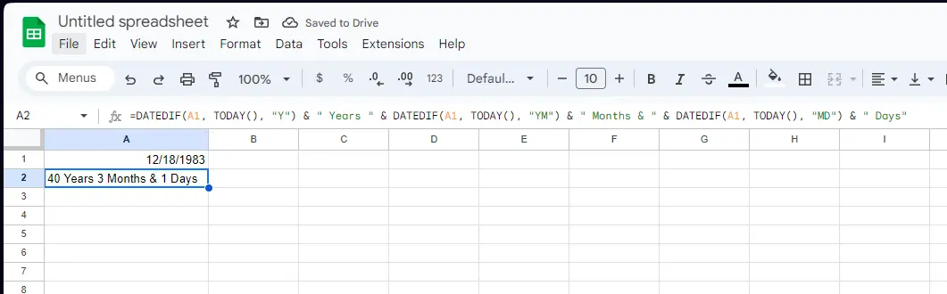
By combining the DATEDIF function with concatenation, you can create a comprehensive age statement in your Google sheet. The formula for a detailed age calculation is:

'=DATEDIF(A1, TODAY(), "Y") & " Years " & DATEDIF(A1, TODAY(), "YM") & " Months & " & DATEDIF(A1, TODAY(), "MD") & " Days"

This formula calculates the total years; the remaining months after subtracting the years; and the remaining days after subtracting the months.

For calculating age across multiple rows simultaneously, the ARRAYFORMULA function can also be used in combination with the DATEDIF formula:

'=ArrayFormula(DATEDIF(A1:A5, TODAY(), "Y") & " Years " & DATEDIF(A1:A5, TODAY(), "YM") & " Months & " & DATEDIF(A1:A5, TODAY(), "MD") & " Days")'

This formula will calculate the age for each DOB listed in cells A1 through A5, displaying the result in a detailed format for each entry.

While more complex, using such formulas allows efficient age calculation from DOB in Google Sheets.