How to find, highlight, and remove duplicates in Google Sheets

Having duplicate data can potentially undermine the quality and accuracy of your performance metrics, sales dashboards, app KPIs, decision-making, and other mission-critical efforts. Therefore, it is essential to have an effective data cleanup method that can identify and eliminate duplicates in Google Sheets.

This blog offers a comprehensive guide with step-by-step walkthroughs and examples of various techniques you can use to highlight duplicates in Google Sheets. Moreover, you may find our video tutorial below to be a valuable resource that provides a complete overview of how to highlight duplicates in Google Sheets.

Try Bardeen to learn to automate with Google Sheets and many more!

Clean and prepare your Google Sheets for highlighting duplicates

Manually copying data is the biggest reason for duplicated and not clean data. If you are still copying data from Salesforce to Google Sheets, or pasting data from LinkedIn to Google Sheets. You should try Bardeen.ai

Bardeen.ai helps you connect Google Sheets with your data sources, so you don’t need to copy and insert data automatically.

Bardeen also connects with ClickUp, Airtable, and 100+ other integrations, and 100+ ready to use websites data scrapers.

Before attempting to highlight duplicates in Google Sheets, try to ensure the following:

• Eliminate other conditional formatting rules currently applied to the cell you’re targeting
• Make sure you don’t have missing spaces in your searches
• Do not select headers when highlighting duplicates with Array Formulas
• Avoid highlighting specified duplicate values if necessary. Select the cells with the conditional formatting rule. Then click the trash icon under Format > Conditional formatting.

Here’s another pitfall to watch out for. Google Sheets can fail to highlight duplicates due to extra space characters.

This is when there are extra spaces — trailing or leading spaces — around the text in one cell but not in another. These extra spaces within the cells can result in missed duplicates, since Sheets searches for an exact match.

You can remove extra spaces in your cells by using the TRIM or CLEAN functions in Google Sheets.

Follow these steps to clean and prepare your Google Sheet to find, highlight and remove duplicates.

1. Trim
2. Clean
3. List
   

6 Ways to find, highlight and remove duplicates in Google Sheets

In Google Sheets, you can use custom formulas paired with conditional formatting to find and highlight duplicates. So that you can remove the duplicates and clean your sheets.

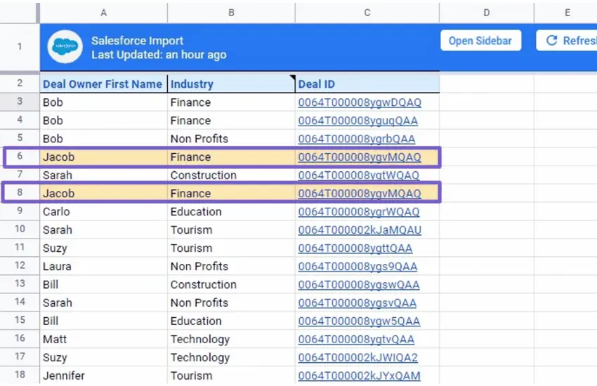
Before we start, let’s pull a sample Salesforce dataset for our examples into Google Sheets. To learn how to import data from Salesforce to Google Sheets in one click with Bardeen.ai, learn more about Salesforce to Google Sheets integration.

Try these ready to use automations:

You can also connect HubSpot, Pipdrive, Notion, Airtable, ClickUp or other CRMs to Google Sheets.

We’ll use this Salesforce dataset to perform the step-by-step walkthroughs below.

1. Formula-free way to highlight duplicates — Remove Duplicates add-on for Google Sheets

Of course, you may have some other use case that requires another formula. Nonetheless, any formula and conditional formatting require a learning curve. If you're not ready to devote your time to those, there's an easier solution.

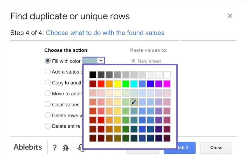
Remove Duplicates add-on for Google Sheets will highlight duplicates for you.

It takes just a few clicks on 4 steps, and the option to highlight found duplicates is just a radio button with a color palette:

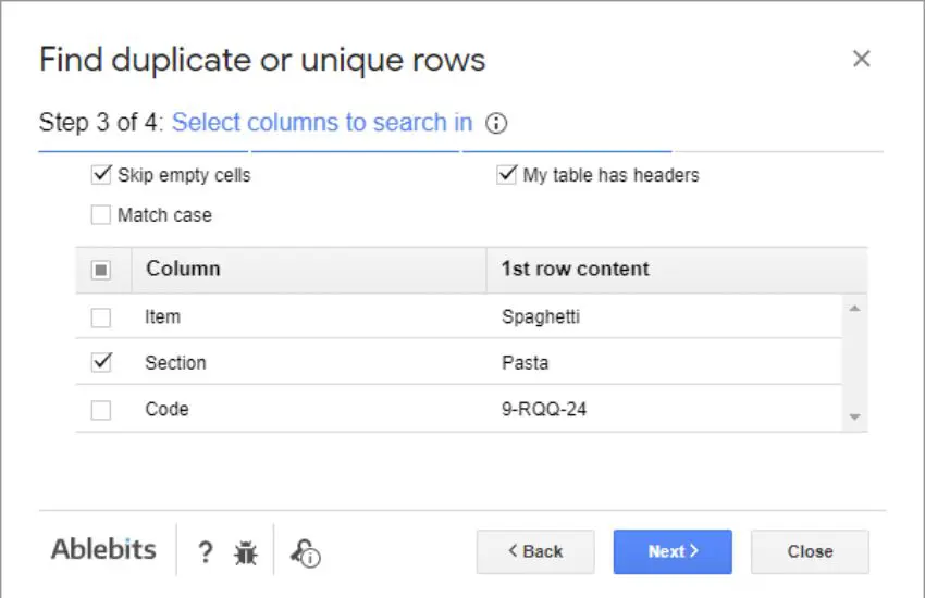
The add-on offers an intuitive way to select your data and pick columns you'd like to check for duplicates. There's a separate step for each action so you won't get confused:

Besides, it knows how to highlight not only duplicates but also uniques. And there's an option to ignore 1st instances as well:

2. Highlight duplicates using the UNIQUE function

Let’s start with the easiest method, using the UNIQUE formula to find all the unique values within a cell range. The function works best with a smaller dataset.

Select an empty cell. Type in =UNIQUE and include the data range you want to check for unique data:

=UNIQUE(B1:B18)

This finds the unique value in B1 to B18

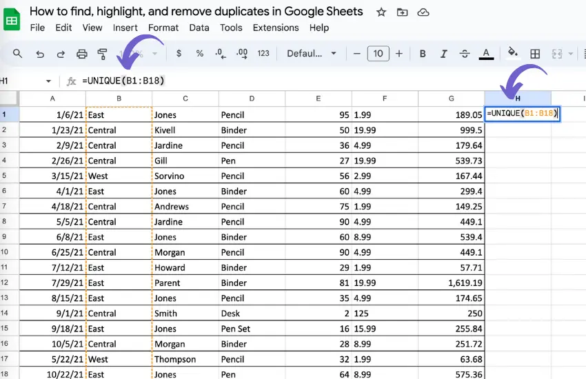
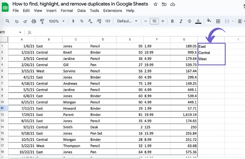
The formula will return the unique values within B1:B18.

UNIQUE eliminates complicated formula configurations and provides you with a clean dataset without duplicates. However, in more advanced duplicate use cases, this function alone can run into limitations.

3. Highlight duplicates in a single column

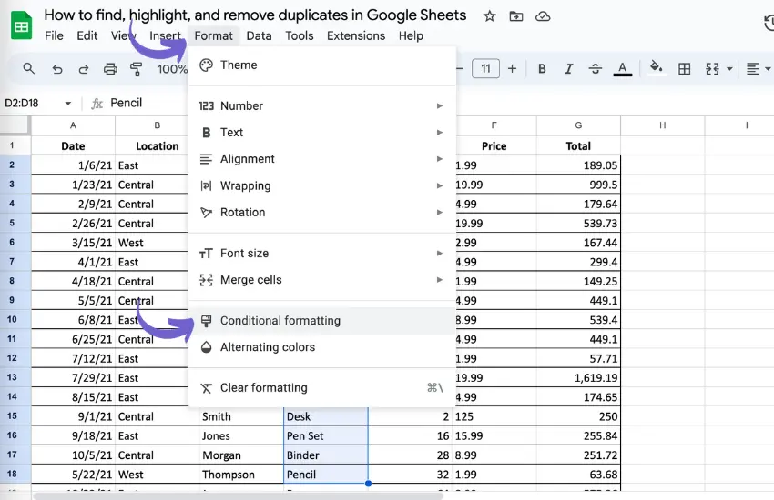
     1. Select the values in the column you want to highlight. It’s important to note that we need to exclude the headers.

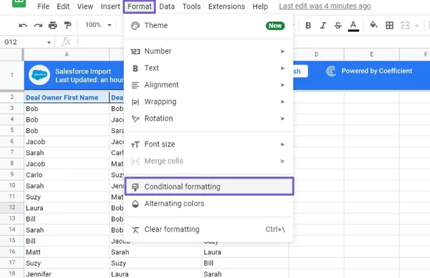
     2. Click Format in the top menu and select Conditional Formatting from the dropdown.

     3. Click Add another rule on the Conditional format rules side panel. If you want to make sure all future new data in these columns are included, you can change the range to C:C.

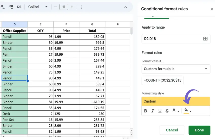
     4. Under Format rules, click Format cells if… and select Custom formula is from the drop down menu.

     5. Enter the COUNTIF formula under the Format cells if… field.

        =COUNTIF($C$3:$C$18,C3)>1

        Please note you need to change the range here if you want to highlight duplicates in a different range. If you want to make sure all future new data in these columns are included, you can change the range to C3:C

     6. Change the the Formatting style options to specify how you want the duplicates to be highlighted. Yellow is my personal go-to, but orange or red also do the trick. You can also use bold, strike or other format options.

        7. Finally, click Done. You will see the duplicate cells highlighted in the column range in your set color and format.

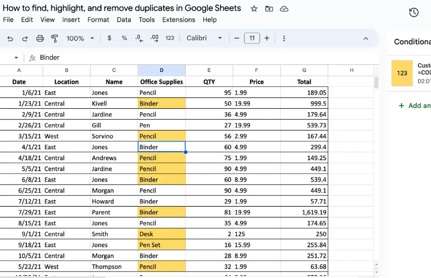
This method uses conditional formatting which means the formatting will update automatically. You only need to setup once, and the highlighting will work in the future even if the data is updated.

You can then review and remove the highlighted duplicate values.

4. Find, highlight and delete duplicates in multiple columns

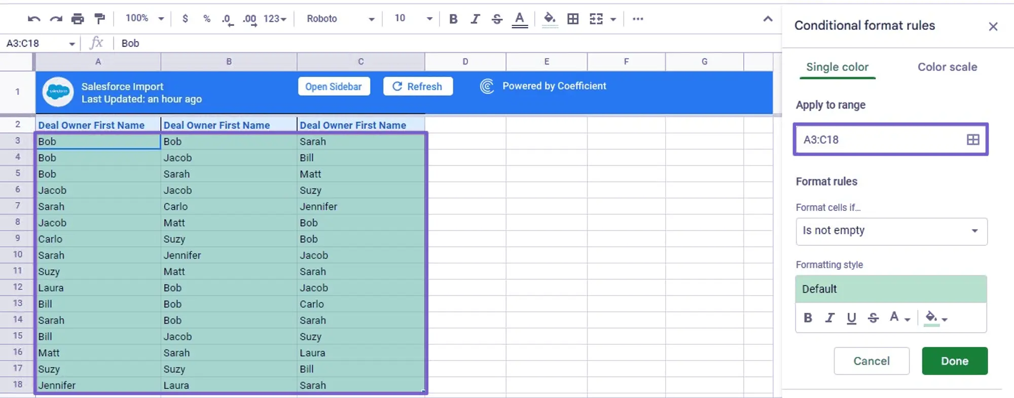
For example, let’s say you have three columns, all containing duplicate data.

     1. The steps to highlight multiple columns are similar to the steps for one column. Select the data range (it’s important to exclude the headers) and click Format > Conditional formatting.

     2. Select Add another rule on the Conditional format rules side panel. Double check the range of cells. Make sure it includes all the columns you want to find duplicates in. If you want to make sure all future new data in these columns are included, you can change the range to A:C

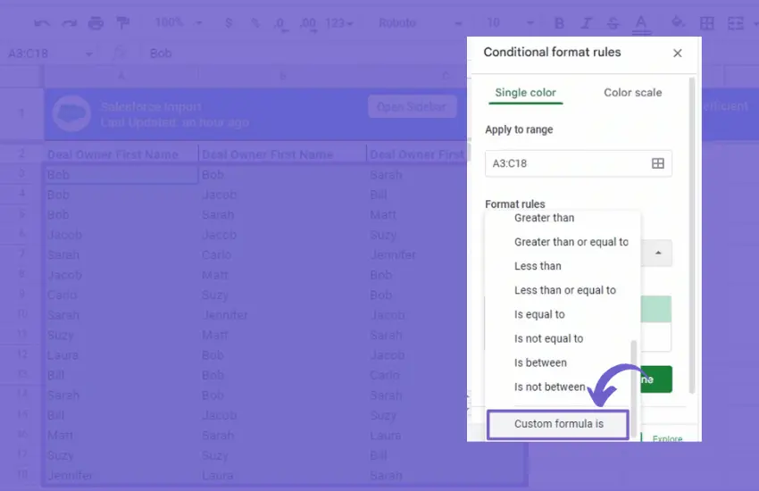
     3. Click the Format cells if… option and select Custom formula is.

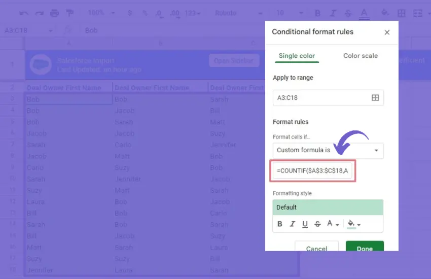
     4. Enter the following formula in the designated field.

         =COUNTIF($A$3:$C$18,A3)>1

If you want to make sure all future new data in these columns are included, you can change the range to A3:C

     5. Set your preference in the formatting style section for highlighting duplicate data and click Done. The duplicate names that appear across these three columns are now highlighted.

     6. You can review and delete the duplicated values

5. Highlight the entire row if duplicates are in one column

Next up is the case when your table contains different records in each column. But the entire row in this table is considered as a single entry, a single piece of information:

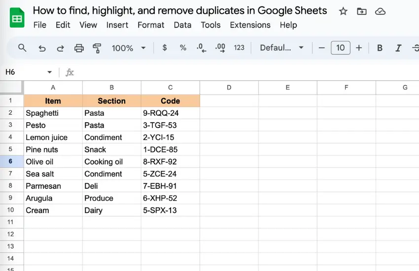
As you can see, there are duplicates in column B: pasta & condiment sections occur twice each.

In cases like this, you may want to treat these entire rows as duplicates. And you may need to highlight these duplicate rows in your Google spreadsheet altogether.

If that's exactly what you're here for, make sure to set these for your conditional formatting:

     1. Apply the rule to the range A2:C10

     2. And here's the formula: =COUNTIF($B$2:$B$10,$B2)>1

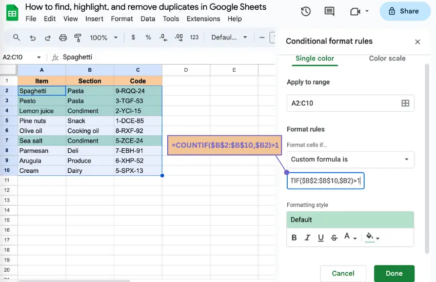
This COUNTIF counts records from column B, well, in column B :) And then the conditional formatting rule highlights not just duplicates in column B, but the related records in other columns as well.

6. Find, highlight and remove duplicate rows

Finding and highlight duplicate rows is slightly less straightforward than highlighting duplicated cells in columns.

This method will highlight the row if the row are duplicated, meaning all selected corresponding cells in the rows contain the same data.

To find duplicate rows, follow the steps from the previous example, but with modifications to the Custom formula is step:

1. Select your data range, but not the header row
   
   
2. Open the Conditional formatting option and the Conditional format rules side panel from the Format top menu
   
   
3. Click Add another rule
   
   
4. Select Custom formula is from the Format cells if… dropdown list
   
   
5. Input the following formula in the Value or formula field:
   
   =COUNTIF(ARRAYFORMULA($A$3:$A$18&$B$3:$B$18&$C$3:$C$18),$A3&$B3&$C3)>1
   
   If you want to make sure all future data in these rows are included, update the range to A3:C by removing the 18
   
   The ARRAYFORMULA part concatenate the values in all cells in a row into 1 single string. And COUNTIF function checks the number of times the combined string repeats in the column.
   
   
6. Choose your preferred formatting style and color for your highlighted duplicates
   
   
7. Click Done. You should see rows six and eight highlighted, since these contain repeating cell values.
   
   
8. Now you can review and delete the duplicated row.

Summary

Use GPT and AI in your Google Sheets

Learn the tips and trips of Google Sheets

Best google sheets add ons

How to automate and integrate Google Sheets