how to convert data to a table in google sheets

Google Sheets is a powerful tool for organizing and analyzing data, but creating visually appealing and functional tables can be a challenge. In this step-by-step guide, we'll show you how to quickly convert your data into a table format in Google Sheets. By following these simple techniques, you'll be able to structure your data effectively, making it easier to manage and present.

Understanding Google Sheets Table Basics

Google Sheets offers a simple way to create tables for organizing and presenting data. While it may not have all the advanced features of Excel's table functionality, Google Sheets still provides the essential tools for creating functional and visually appealing tables.

Here are the key aspects of tables in Google Sheets:

• Formatting options for header rows, including bold text, center alignment, and text wrapping
• Alternating row colors to improve readability
• Customizable cell formatting, such as number formats, date formats, and text alignment
• Ability to apply filters to columns for quick data analysis

Efficiently organizing your data in a well-structured table is crucial for effective data manipulation and presentation. By taking advantage of Google Sheets' table features, you can create professional-looking tables that make your data easier to understand and work with.

For advanced features, consider adding ChatGPT to Google Sheets for enhanced data analysis and automation.

Preparing Your Data for Table Conversion

Before converting your data into a table format in Google Sheets, it's essential to ensure that your data is well-structured and clean. This will make the table conversion process smoother and help you avoid potential issues down the line.

Here are some tips for preparing your data:

1. Sort your data: Arrange your data in a logical order, such as alphabetically or chronologically, to make it easier to read and analyze.
2. Align your data: Ensure that each column contains the same type of data (e.g., text, numbers, or dates) and that the data is consistently formatted.
3. Categorize your data: Group related data together and use clear, descriptive headers for each column.
4. Remove duplicates: Check for and remove any duplicate entries to avoid skewing your analysis.
5. Fix inconsistencies: Look for inconsistent data, such as variations in spelling or formatting, and standardize them.

Google Sheets offers a helpful feature called "Cleanup Suggestions" that can assist you in identifying common errors, such as extra spaces, duplicates, or inconsistent data. To access this feature, click on "Data" in the menu, then "Data cleanup," and finally "Cleanup suggestions."

You can connect Google Docs with Bardeen to automate your data preparation tasks and save time.

By taking the time to properly structure and clean your data before converting it into a table, you'll set yourself up for success when it comes to data analysis and presentation.

Using the 'Alternating Colors' Feature to Create Table-like Structures

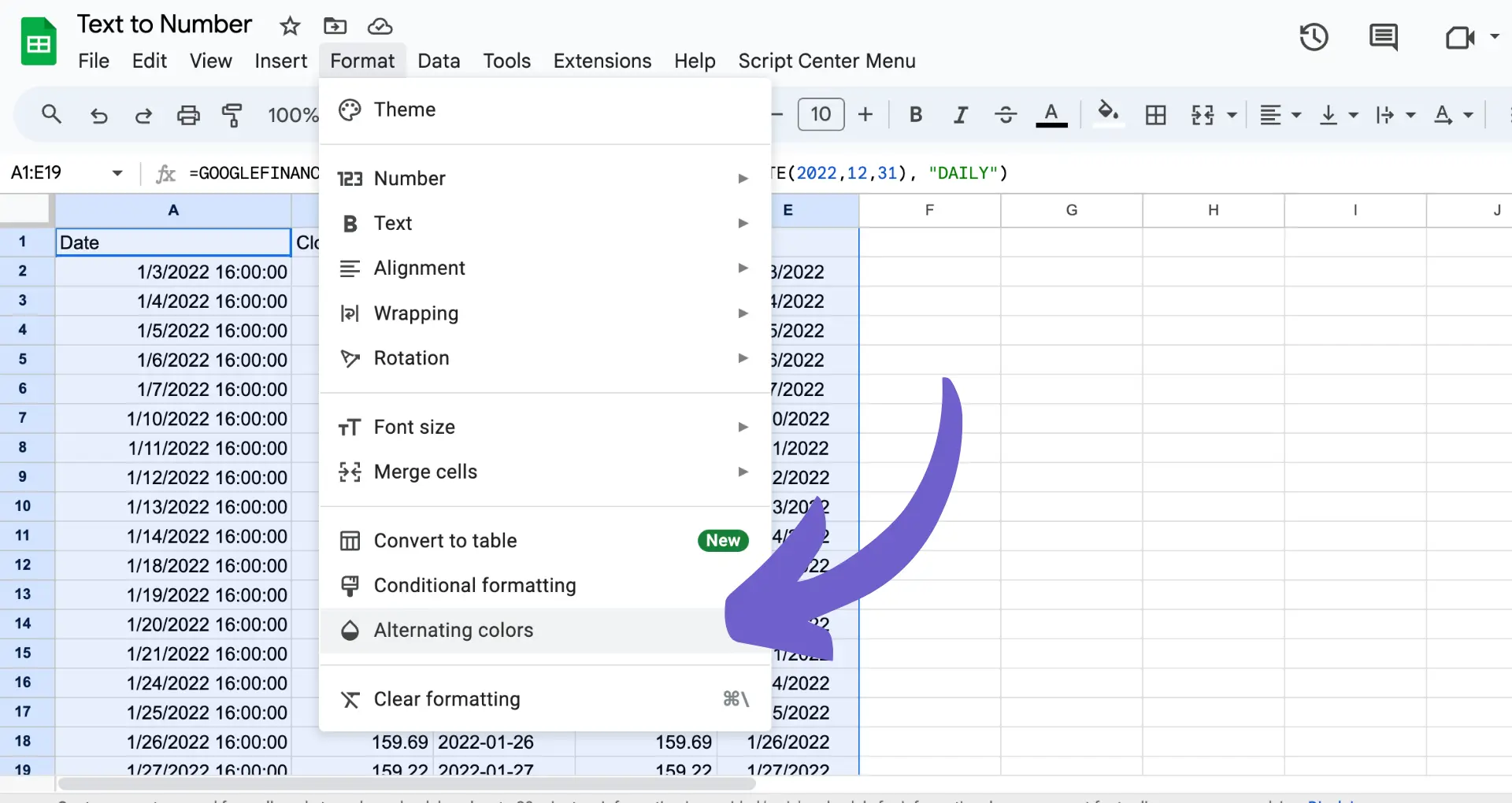
Google Sheets offers a handy feature called 'Alternating Colors' that allows you to visually distinguish data rows, simulating a table format. This feature is particularly useful when working with large datasets, as it makes it easier to read and interpret the information.

Here's a step-by-step guide on how to use the 'Alternating Colors' feature:

1. Select the range of cells you want to format as a table.
2. Click on the 'Format' menu in the toolbar and hover over 'Alternating colors.'
3. Choose a pre-designed color scheme from the options provided, or click on 'Custom alternating colors' to create your own.
4. If you opted for a custom color scheme, select the colors you want to use for the header, first row color, and second row color.
5. Click 'Done' to apply the alternating colors to your selected data range.

You can further customize the appearance of your table by adjusting the cell borders, font styles, and alignment. To do this, simply select the formatted data range and use the formatting options in the toolbar.

By applying alternating colors to your data, you can create a visually appealing table-like structure that makes it easier to analyze and present your information effectively. For more advanced features, check out GPT in Spreadsheets to enhance your Google Sheets experience.

Implementing Filters for Enhanced Data Management

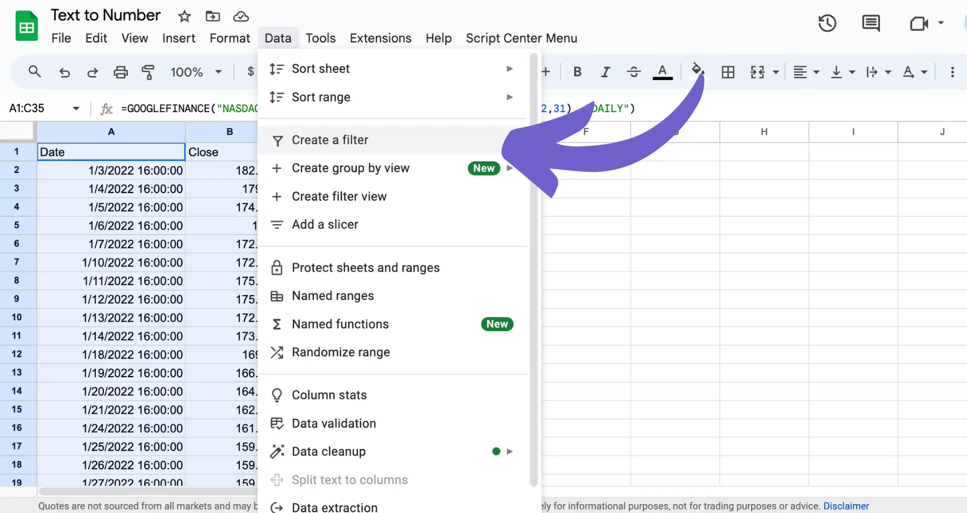
Filters in Google Sheets provide a powerful way to manage and analyze your table data more efficiently. By adding filters to your columns, you can quickly sort, search, and hide specific data points, making it easier to focus on the information that matters most.

Here's how to add filters to your Google Sheets columns:

1. Select the range of cells you want to filter, including the header row.
2. Click on the 'Data' menu in the toolbar and select 'Create a filter.'
3. You will now see filter icons (upside-down triangles) next to each column header in your selected range.
4. Click on a filter icon to open the filter options for that column.
5. Choose from the various filter options, such as sorting, searching, or filtering by condition, value, or color.
6. Click 'OK' to apply the filter to your data.

Using filters offers several benefits, particularly when working with large datasets:

• Quickly locate specific data points or patterns within your table.
• Hide irrelevant data temporarily, allowing you to focus on the information you need.
• Easily sort your data by various criteria, such as alphabetical order, numerical order, or custom conditions.
• Apply multiple filters simultaneously to create more complex data views.

By leveraging the power of filters in Google Sheets, you can significantly improve your data accessibility and analysis capabilities, saving time and effort in the process. Additionally, you can integrate Excel with Bardeen to automate sequences of actions, making your workflows faster and more efficient.

Use Bardeen to enrich LinkedIn profile links in your Google Sheets. Stay focused on important tasks while automating tedious data work with a click.

Advanced Formatting Options for Tables in Google Sheets

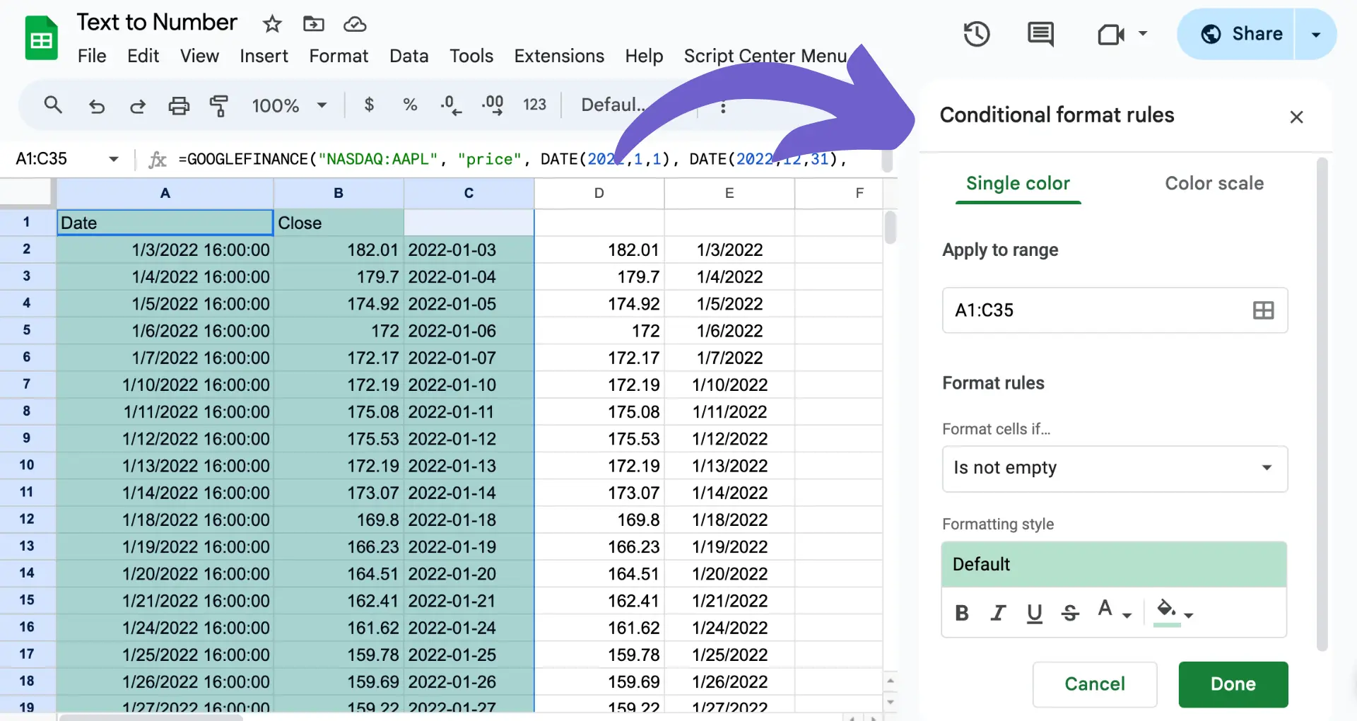
Google Sheets offers several advanced formatting techniques that can help you highlight key data and reduce errors within your tables. One such technique is conditional formatting, which allows you to dynamically format cells based on specific criteria.

To apply conditional formatting:

1. Select the range of cells you want to format.
2. Click on "Format" in the menu bar and choose "Conditional formatting."
3. Set the rules for your formatting, such as highlighting cells that contain values greater than a certain number or fall within a specific range.
4. Choose the formatting style (e.g., background color, font color, or custom formatting) to apply when the conditions are met.

Another useful tool for improving data accuracy and consistency in your Google Sheets tables is data validation. This feature allows you to restrict the type of data that can be entered into specific cells, reducing the risk of input errors.

To set up data validation:

1. Select the cells you want to validate.
2. Click on "Data" in the menu bar and choose "Data validation."
3. Set the criteria for valid data, such as a list of predefined options, a specific number range, or a custom formula.
4. Optionally, provide input messages to guide users and error alerts to notify them of invalid entries.

Named ranges can also be used within tables to make formulas more readable and easier to apply. By assigning a meaningful name to a range of cells, you can reference that name in formulas instead of using cell references.

To create a named range:

1. Select the cells you want to name.
2. Click on "Data" in the menu bar and choose "Named ranges."
3. Enter a name for the range and click "Done."
4. Use the named range in formulas by typing its name instead of the cell references.

By leveraging these advanced formatting options, you can create visually appealing and error-resistant tables in Google Sheets, making your data more accessible and actionable.

Automating Table Updates with Google Sheets Functions

Google Sheets offers a range of powerful functions that can help automate data updates within tables, reducing the need for manual entry and saving you time. Two particularly useful functions for this purpose are ARRAYFORMULA and QUERY.

The ARRAYFORMULA function allows you to apply a formula to an entire range of cells, automatically expanding the formula as new data is added. This means you can set up calculations or transformations once, and they will be applied to new rows or columns without the need for manual copying or dragging.

For example, if you have a table with sales data and want to calculate the total revenue for each row, you can use ARRAYFORMULA like this:

=ARRAYFORMULA(B2:B * C2:C)

This formula multiplies the values in column B (price) by the values in column C (quantity) for all rows, starting from row 2. As new sales data is added, the total revenue will be automatically calculated for each new row.

The QUERY function is another powerful tool for automating table updates. It allows you to perform database-like operations on your data, such as filtering, sorting, and aggregating, using a simple SQL-like syntax.

For instance, if you want to create a summary table that shows the total revenue by product category, you can use QUERY like this:

=QUERY(A2:D, "SELECT A, SUM(D) GROUP BY A LABEL SUM(D) 'Total Revenue'")

This formula selects data from the range A2:D, groups the data by the values in column A (product category), and calculates the sum of the values in column D (total revenue) for each group. The result is a new table with product categories and their corresponding total revenue, which updates automatically as new data is added to the original table.

By leveraging functions like ARRAYFORMULA and QUERY, you can create dynamic, self-updating tables in Google Sheets that save you time and ensure your data is always up-to-date. To further boost your productivity, consider automating outreach with tools like Bardeen.

Bardeen makes automating tasks simple. Learn more about using Google Drive with other apps to keep your files organized and reduce time spent on manual updates.