Like most Google products, Google Sheets is popular thanks to its easy accessibility and live collaboration features. But do you know about the ‘Explore’ feature, how to check column graphs at a glance, or how to create quick ‘Sparkline’ graphs? Or how to add AI or ChatGPT to Google Sheets?
These are the features that can make you a Pro in Google Sheets, and most people don’t even know they exist. In this article, we’ll look at 21 exciting Google Sheets tips and tricks to improve your workflow, better visualize data, and save time!
Before we dive into the tips and tricks, let’s take a minute to talk about Bardeen. An AI workflow automation extension in Chrome, it’s integrated with Google Sheets. Install it for free.
Since Bardeen is integrated with other apps, it’ll also allow you to connect Google Sheets with third-party apps and perform automations. From copying LinkedIn job details to saving Instagram followers, all of it is made possible by Bardeen! We’ll talk more about these automations in the article. Now, let’s dive into the list.
Saving time is one of the main reasons you clicked on this article! Here are three tips that’ll help you save a lot of time when using Google Sheets.
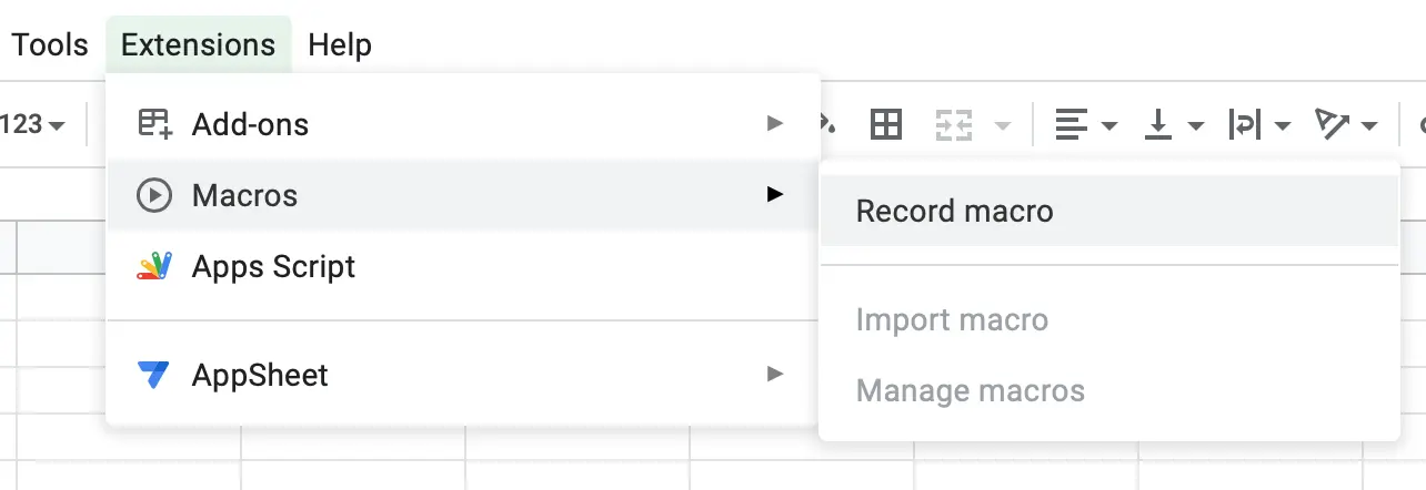
Do you often find yourself performing the same set of actions in a spreadsheet on Google Sheets? Macros will allow you to record and then automate those steps! In the menu bar, go to Extensions and click on Macros. You can record a macro, import one, or manage all your existing ones here.
This can be useful to automate repetitive tasks, but it’s limited to only one Google Sheet. To learn more about macros and the steps to implement them into a spreadsheet, check out this article.
Since your hands are generally rested on the keyboard when using a computer, knowing a few keyboard shortcuts can save you a lot of time. You can easily access a searchable list of keyboard shortcuts in Google Sheets. Just press Ctrl (Command on Mac) and Forward Slash.

You can click on View Compatible Shortcuts and toggle on Enable compatible spreadsheet shortcuts if you want to view relevant keyboard shortcuts based on if you’re using Windows, Mac, or Chrome OS.
As you can see, there are many useful keyboard shortcuts for editing, accessing menus, formatting, and managing data. Be sure to get familiar with these, and start introducing them into your workflow to save time!
If macros are too limited for your use case, there are some automation platforms you can look into. These platforms are integrated with the Google Sheets API and let you connect it to other apps and perform automations.
In addition to Google Sheets, Bardeen is also integrated with Slack, Notion, ClickUp, and many other apps.
With its AI capabilities, Bardeen can also understand your data, create content, and even create your automations within a few clicks. Thanks to this, you can create your own automations or use pre-made ones to connect Google Sheets with other apps! If you’ve installed it, here are a few automations you can try out.
What makes Bardeen special among most automation platforms is that it can connect OpenAI with Google Sheets. To learn more about other Bardeen automations for Google Sheets! Elevate your Google Sheets with ChatGPT and AI.
Once you’ve learned how to save time in Google Sheets by automating repetitive tasks and finding shortcuts, it’s time to boost your productivity further! Here are three tips to boost your productivity in Google Sheets.
If you’ve highlighted a set of cells and want to view statistics that can help you make heads and tails of that data, Google Sheets provides a great way to do that. First, make sure to select the range that you want to analyze. Then, click on Data in the menu bar and Column stats.

As an example, we’re using Google’s ‘Explore example’ spreadsheet here. There are many stats you can view, like sum, average, and median. You can also switch to other columns if you want to view those stats.
The above tip is useful if you want to dive deep into some data, but what if you want to quickly check the sum count of numbers in a column? There’s a quick way to check it in Google Sheets! Once you’ve highlighted all the numbers in a column, just check the bottom-right corner of the window.
If you click on the sum, you can also view the average, minimum, and maximum. Say, if you only want to view the maximum, you can click on it too. Next time you highlight a column of numbers, you’ll be shown the maximum by default.
Whether you want to translate text (‘=GOOGLETRANSLATE’) or import a table from the Internet (‘=IMPORTHTML’), we all love functions in Google Sheets! It’s even possible to wrap a function around another function. Here’s an example:
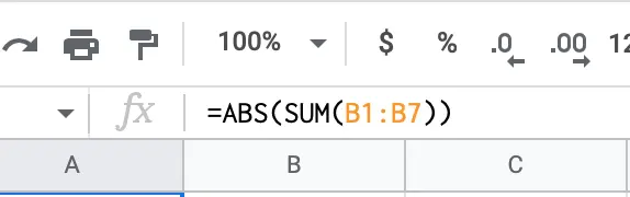
When you write it this way, remember that Google Sheets executes the inner function first, which is also called a nested function. In Google Sheets, when you start typing a new function, you’re also shown a few details about it.

If you want to learn all functions from A to Z, this page includes names, syntax, and descriptions.
One of the biggest benefits of Google Sheets is that it’s easily accessible and updated in real-time. This makes it optimal for collaboration, so let’s explore three tips to share Google Sheets.
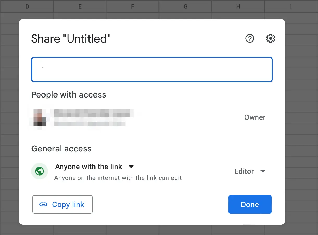
If you don’t want to manually invite each member of your team to your spreadsheet, you can instead copy a link to let them access it. Click the Share button at the top-right corner of the window.
In the pop-up window, click on Restricted and choose Anyone with the link. A drop-down menu will appear where you can designate the role of any person who opens the link: Viewer, Commentator, or Editor. Once you choose the right options, click Copy link and share that link with your team!
When a user opens your spreadsheet, do you want to pull their attention to a certain set of cells? Highlight the column or row you want to share, right-click it, click on View more cell actions, and click Get link to this range. When they open the link, the range will be highlighted for them.
Do you want others to make their own copy of the spreadsheet and edit it independently? Open the spreadsheet in your browser and copy the link from the address bar. In the link, change ‘edit’ to ‘copy’ instead. Whoever clicks this link will be given the option to make their own copy of the spreadsheet.

Here’s another cool tip! If you just want a direct download link to your spreadsheet, replace ‘edit’ in the link with ‘export?format=csv’ or ‘export?format=pdf’ instead, depending on the file type you want to share. When anybody opens the link, they can download the spreadsheet.
If you want to protect a range of cells, highlight them, right-click, and go to View more cell actions. From the drop-down menu, click on Protect this cell range. If you want to protect a sheet, right-click on it and choose Protect sheet.
Once you’ve entered a description and specified which cells or sheets you want to protect, click on Set permissions. You can either choose to show a warning every time someone tries to edit that part of the spreadsheet or restrict it entirely to only yourself and certain team members.
Since you’ve made your spreadsheet accessible to anyone with a link, you can now even embed it on a website! Go to the menu bar and click on File > Share > Publish to Web.
In the pop-up window, you’ll see two tabs: Link and Embed. If you just want a publicly-accessible link to the spreadsheet, go to the Link tab. If you want to embed the spreadsheet to a website, go to the Embed tab. You also have all the necessary options for what data you want to display!
Bonus Tip: Within the Google suite, there are many features in place that let you connect Google Sheets with other apps. In Google Docs, you can insert a chart from Google Sheets. In a Doc, click on Insert in the menu bar, Chart, and From Sheets. Whenever a new form is submitted in Google Forms, you can also have the data sent directly to a Google Sheets spreadsheet as a new row. Click here for more info.
When collaborating with others on a spreadsheet, comments are useful for communication. If you add a comment and want to ensure that a certain team member gets notified of it, here’s a handy tip you can use.
Type out the comment as you normally would, but at the end of it use the ‘+’ or ‘@’ symbol. This will display your email directory in a drop-down menu. Type in the name or email address of the person you want to share the comment with and press Enter. You also get the option to assign them that comment.
Importing data from other apps into Google Sheets can often be a tedious process. Fortunately, Bardeen offers many ready-to-use automations which let you copy data from other apps to Google Sheets in just one click. Here are a few such automations you can try out!
Notion database is convenient, but can't do calculations or pivot tables. This playbook exports Notion database to Google Sheet with 1 click. Explore more Google Sheets and Notion integrations.
Easily export and sync data between ClickUp and Google Sheets with this playbook. Or explore more Google Sheets and ClickUp integrations.
Based on your use case, some of the above automations can help you skip hours of copy-pasting! You can check out more Bardeen automations.
Data visualization is one of the core purposes of creating a spreadsheet. Google Sheets has many useful features that help you break down your data to gain insights and catch patterns. Let’s look at three tips for data visualization!
Pie and bar graphs make data easier to understand, but take up a lot of space. Instead, the ‘=SPARKLINE’ formula allows you to create a single-cell graph. Click on the cell where you want to insert a Sparkline graph, then type ‘=SPARKLINE’ and open parenthesis and highlight the data range.
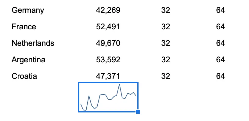
By default, it’ll use a line graph, but it’s also capable of a bar, column, and win-loss chart. Check this page for advanced functions.
It’s not always easy to come up with ideas for formatting and analyzing your data. To get your creative juices flowing, Google Sheets has the ‘Explore’ feature.
It can work for all the data in your spreadsheet, but you can also highlight a range of cells if you want info for specific data. To open it, go to the bottom-right part of the window and click on the Explore button.
A side panel will open up. The coolest part here is that you can ask it questions about the data in your spreadsheet! Under Answers, you can type a question in the text box (like ‘Total Profit in November 2023’) or choose from a list of suggestions.
Scroll below, and you'll find some charts and a pivot table for the data. If you want to add one, you can just drag it to your spreadsheet. You can also add alternating color backgrounds to change the look of your spreadsheet.
If you’re creating a spreadsheet for sales every month, wouldn’t it be great if cells with profit are highlighted in green and cells with loss in red? That’s the power of conditional formatting!
Once you highlight all the cells you want to add conditional formatting to, click Format in the main menu and Conditional Formatting. A side panel will open up where you can specify the conditions for the formatting of those cells.
We tend to grasp color tones much easier than raw numbers. If you want to add a varying color tone to higher and lower values in your cells, you can click on the Color scale tab.
Your spreadsheet might have all the data you need, but it needs to be organized properly for it to be understandable. So, finally, let’s discuss some tips to organize spreadsheets.
Is there a column in your spreadsheet that is just limited to specific values, like Passed and Failed, or Yes and No? You can constrain what data you can input in specific cells to make things more organized.
First, highlight the range of cells where you’d like to do this, click on Data in the main menu, and Data Validation. A side panel will open. Under Criteria, you can choose to create a dropdown or checkbox for that range of cells!
This might seem like a bit of work, but it can save you from the pain of typing something repeatedly and also lowers the chances of errors.
When working in a large spreadsheet, it can be useful to be able to filter your data. Click on Data in the menu bar and Create a filter. A filter icon will be added next to all column headers.

Google Sheets has also recently launched the Slicer feature. Learn more about it in this video.
All in all, adding filters to your spreadsheet can make it easier to parse through data and gain insights!
When data is transferred from one spreadsheet to another, it’s likely that it can end up with some unnecessary characters and extra spaces. This can make your spreadsheet look messy and interfere with data processes.
The ‘=CLEAN’ and ‘=PROPER’ functions are worth trying out to remove non-printable characters and capitalize names. In addition, you can use the ‘=SPLIT’ function to separate first and last names into different cells.
For further suggestions on cleaning up your spreadsheet, click on Data in the menu bar and go to Data cleanup. Here, you’ll find the Cleanup suggestions, Remove duplicates, and Trim whitespace options!
If you’d like to be able to view the headers of each column as you scroll down your spreadsheet, you can freeze the header row in Google Sheets. First, select the row you want to freeze, then click View, Freeze, and 1 row.

Now, as you scroll through your spreadsheet, the header will stay pinned at the top, like this.
If you want to distinguish a range of cells from the rest, adding a border to them will do the trick. To do this, highlight the cells, click on the Borders icon, and choose which side you want to add a border to.
In addition, you can also change the border color and style if you want.
Making a spreadsheet look great is just as important as organizing it well. To save you time, Google Sheets includes many themes to revamp your spreadsheet instantly. Click on Format in the menu bar and Theme.
Beyond using a theme, you can also use a template. Check out the Template gallery on the homepage to view all default templates. We have also created a content calendar and weekly calendar template. Plus, be sure to check out Vertex42 and Smartsheet for some great templates!
Sometimes you might paste a link or sentence that doesn’t fit in a single cell. You can wrap it inside a column. Click Format in the menu bar and Wrapping. You can choose from three options: Overflow, Wrap, and Clip.
One of the biggest benefits of Google Sheets is that it offers you the ability to download extensions and add-ons. These can give you access to new features and push the boundaries of what’s possible with Google Sheets.
Two popular Google Sheets add-ons are Google Analytics and Supermetrics. There are many more add-ons in the Google Workplace Marketplace. We'll talk more about Google Sheet add-ons in an upcoming article!
Yes! This can have many benefits, like automation and better access to data. Learn how to create your own calendar in Google Sheets.
So, here we are! These were 21 tips and tricks for Google Sheets. Of course, almost everybody knows how to use Google Sheets, but being knowledgeable about these features can make you look like a true professional.
This doesn’t cover everything you can do with Google Sheets. In upcoming articles, we’ll explore Google Sheets formulas and add-ons, so stay tuned for that!
For now, try out a few of these tips and see how it goes! There’s always the Undo button if you make a mistake.
If you’re migrating from Notion to Google Sheets, Bardeen can help you skip all the copy-pasting!


SOC 2 Type II, GDPR and CASA Tier 2 and 3 certified — so you can automate with confidence at any scale.